Team Member:
- Nadira Amadou
- Oluwatofunmi Sodimu
- Thanapol Tantagunninat
This project is inspired by the following competition: Kelp Wanted: Segmenting Kelp Forests
Introduction/Problem Definition:
A kelp forest is an ocean community made up of dense groupings of kelps. These forests typically serve as a source of food, shelter, and protection to a wide variety of marine life [1]. Moreover, the significance of kelp forests extends beyond their role as a biodiverse hotspot. They play a pivotal role in regulating marine environments and supporting human well-being. Kelps are renowned for their capacity to sequester carbon dioxide through photosynthesis, contributing significantly to carbon capture from human’s daily life and carbon storage in the oceans [2]. Additionally, these underwater havens act as natural buffers against coastal erosion, mitigating the impacts of waves and currents on shorelines. Furthermore, kelp forests hold economic value, serving as crucial fishing grounds and tourist attractions in many coastal regions.
However, these forests face threats from multitude of factors such as climate change, acidification, overfishing, and unsustainable harvesting practices [1].
To address these pressing conservation concerns and safeguard the future of kelp forests, innovative approaches are needed. One promising strategy involves harnessing the power of technology to monitor and protect these vital marine habitats. By leveraging advances in remote sensing, computer vision, and machine learning, we propose the development of a comprehensive model capable of monitoring kelp forests using coastal satellite imagery. Such a model would enable tracking of changes in kelp abundance, empowering conservation efforts and informing sustainable management practices. The successful predictions and ongoing automated monitoring can empower authorities, policymakers, and marine conservation organizations to make informed decisions about actions necessary for the preservation of coastal ecosystems.
We aim to develop a kelp segmentation model based on a Convolutional Neural Network (CNN). The input to our model is the satellite images of 350x350 pixels containing 7 channels including Short-wave Infrared (SWIR), Near Infrared (NIR), Red (R), Green(G), Blue (B), Cloud Mask, and Elevation (Ground Mask) of which we will experiment with different selections/combinations of channels as the input to the neural networks. The output/results are the predicted labels that represent the pixels containing kelp (1) or no kelp (0). The goal is to successfully match the predicted kelp labels with the ground truth label in the dataset we used to validate our performance with more than 0.5 Dice coefficient.
Related Works:
[4] Artificial intelligence convolutional neural networks map giant kelp forests from satellite imagery
The paper suggests the use of a Mask R-CNN (mask region-based convolutional neural network) to detect giant kelp forests along the coastlines of Southern California and Baja California using satellite imagery. The authors aimed to develop a more robust and accurate method for detecting kelp forests that can overcome the challenges posed by cloud cover using a mask RCNN. They used a mask RCNN architecture for giant kelp identification and segmentation because it successfully combines the high-performance algorithms of Faster R-CNN for target identification and FCN for mask prediction, boundary regression, and classification.
To solve this problem, they optimize the mask R-CNN model through hyperparameterization. Model hyper-parameterization was tuned through cross-validation procedures testing the effect of data augmentation, and different learning rates and anchor sizes. The optimal model achieved impressive results, with a Jaccard’s index of $0.87 \pm 0.07$, a Dice index of $0.93 \pm 0.04$, and an over-prediction rate of just 0.06. The loss function used in the model is defined by the combination of Classification Loss, Bounding Box Regression, and Mask Loss where the Classification Loss and Bounding Box Regression Loss are determined through cross-entropy as in the Faster R-CNN framework31,32, and reflect the ability of the model to classify kelp and to identify the regions of the image (i.e., bounding boxes) where kelp occurs. The Mask Loss is determined through binary cross-entropy per pixel34, for the images where kelp was classified, and reflects the ability of the model to identify the masks (i.e., the outlines) of kelp forests.
The authors show that their approach can effectively detect kelp forests, even in the presence of occasional clouds, and provide a valuable tool for monitoring and studying these important marine ecosystems. This work advances the state-of-the-art in remote sensing and computer vision techniques for kelp detection and can be applied to other similar applications in the future. Our work aimed to address the challenges of this paper defined by the potential interference of occasional clouds in the detection of kelp forests due to changes in reflectance and the high variability in the spatial patterns of kelp forests.
[5] Automated satellite remote sensing of giant kelp at the Falkland Islands (Islas Malvinas):
- The paper evaluates two methods to automate kelp detection from satellite imagery: 1) crowdsourced classifications from the Floating Forests citizen science project (FF8), and 2) an automated spectral approach using a decision tree combined with multiple endmember spectral mixture analysis (DTM).
- Both methods were applied to classify kelp from Landsat 5, 7, 8 imagery covering the Falkland Islands from 1985-2021.
- DTM showed better performance than FF8 when validated against expert manual classifications of 8 Landsat scenes covering over 2,700 km of coastline.
- Multiple Endmember Spectral Mixture Analysis (MESMA) is a spectral unmixing algorithm that estimates the fractional contributions of pure spectral endmembers (e.g. water, kelp, glint) to each image pixel spectrum based on a linear mixing model. It allows estimating partial kelp coverage within pixels.
- Decision Tree Classification is used to first identify potential candidate kelp-containing pixels before applying MESMA. The decision tree uses spectral rules to separate kelp from non-kelp pixels. Then MESMA spectral unmixing is utilized to estimate fractional kelp coverage within those candidate pixels
[6] Mapping bull kelp canopy in northern California using Landsat to enable long-term monitoring
- This paper is focused on the mapping and monitoring of kelp, specifically bull kelp, though the use of Landsat satellite images.
- Similar to our previous reference, MESMA was used to predict the presence of bull kelp biomass.
- This paper discusses the influence of water endmember quantity and the use of giant kelp versus bull kelp endmembers on the accuracy of MESMA; tidal influence on bull kelp canopy areas; and performs a comparison of the use of Landsat images versus other surveys. The researchers were able to conclude that:
- The number of water endmembers does not significantly influence MESMA performance.
- Bull kelp specific endmembers outperform repurposed giant kelp endmembers.
- Tidal phases do not significantly influence the detection of bull kelp canopy areas.
- Compared to aerial imagery and private satellite images that have been employed by other researchers, Landsat images allow for long-term montioring since they are updated by the U.S. Geological Survey (USGS) every 16 days.
[7] Automatic Hierarchical Classification of Kelps Using Deep Residual Features
This paper presents a binary classification method that classifies kelps in images collected by autonomous underwater vehicles.
The paper shows that kelp classification using classification by deep residual features DRF outperforms CNN and features extracted from pre-trained CNN such as ImageNets. The performance was demonstrated using ground truth data provided by marine experts and showed a high correlation with previously conducted manual surveys. The metrics evaluated were: F1 score, accuracy, precision, and recall.
A binary classifier is trained for every node in the hierarchical tree of the given problem and deep residual networks (ResNets) are extracted to improve time efficiency and the automation process of detection of kelp marine species.
Furthermore, color channel stretch was used on images to reduce the effect of the underwater color distortion phenomenon. For feature extraction, a pre-trained Resnet 50 was used, and the proposed method was implemented using MatConvNet and the SVM classifier. Despite DRF allowing the comparison of kelp coverage in different sites, the proposed method had the drawback of an over-prediction of kelp at high percentage cover and under-prediction at low coverage, even though the prediction was negligible in some sites.
[8] Submerged Kelp Detection with Hyperspectral Data
This paper focuses on the detection of submerged kelp using hyperspectral AisaEAGLE data. The authors propose their solution as an alternative to other kelp mapping approaches that use reflectance-based classification methods and are thus limited in their ability to detect kelp below a certain depth. The proposed solution incorporates an anomaly filter for filtering out any effects on the water surface, an algorithm for kelp feature extraction, and the use of specific spectral features of kelps for identifying pixels with kelp.
Methods/Approach:
Method Overview:
Current best approach.
In our previous work, we explored 2 distinctive model architectures (UNET, CNN). The Unet model performed better than the CNN architectures. In our final work, we build upon the UNET architecture by tuning the hyperparameters of the model and testing numerous data augmentation techniques consisting of combining different channels from the NDVR images provided for the sake of the project.
Architecture Description:
The UNET architecture used in this project is building off of an existing architecture provided by a Paperspace blog on UNET. Table [1] shows the architecture of the model.
| Layer (type) | Output Shape | Param # | Connected to | |
|---|---|---|---|---|
| input_1 (InputLayer) | [(None, 350, 350, 3 )] | 0 | [] | |
| conv2d (Conv2D) | (None, 350, 350, 64 ) | 1792 | [‘input_1[0][0]’] | |
| batch_normalization (BatchNormalization) ) | (None, 350, 350, 64 | 256 | [‘conv2d[0][0]’] | |
| re_lu (ReLU) | (None, 350, 350, 64 ) | 0 | [‘batch_normalization[0][0]’] | |
| conv2d_1 (Conv2D) | None, 350, 350, 64) | 36928 | [‘re_lu[0][0]’] | |
| batch_normalization_1 (BatchNormalization ) | (None, 350, 350, 64) | 256 | [‘conv2d_1[0][0]’] | |
| re_lu_1 (ReLU) | (None, 350, 350, 64) | 0 | [‘batch_normalization_1[0][0]’] | |
| max_pooling2d (MaxPooling2D) | (None, 70, 70, 64) | 0 | [‘re_lu_1[0][0]’] | |
| conv2d_2 (Conv2D) | (None, 70, 70, 320) | 184640 | [‘max_pooling2d[0][0]’] | |
| Batch_normalization_2 (BatchNo rmalization) | (None, 70, 70, 320) | 1280 | [‘conv2d_2[0][0]’] | |
| re_lu_2 (ReLU) | (None, 70, 70, 320) | 0 | [‘batch_normalization_2[0][0]’] | |
| conv2d_3 (Conv2D) | (None, 70, 70, 320) | 921920 | [‘re_lu_2[0][0]’] | |
| batch_normalization_3 (BatchNormalization) | (None, 70, 70, 320) | 128 | [‘conv2d_3[0][0]’] | |
| re_lu_3 (ReLU) | (None, 70, 70, 320) | 0 | [‘batch_normalization_3[0][0]’] | |
| max_pooling2d_1(MaxPooling2D) | (None, 14, 14, 320) | 0 | [‘re_lu_3[0][0]’] | |
| conv2d_4 (Conv2D) | (None, 14, 14, 1600) | 4609600 | [‘max_pooling2d_1[0][0]’] | |
| batch_normalization_4 (BatchNo rmalization) | (None, 14, 14, 1600 | 6400 | [‘conv2d_4[0][0]’] | |
| re_lu_4 (ReLU) | (None, 14, 14, 1600) | 0 | [‘batch_normalization_4[0][0]’] | |
| conv2d_5 (Conv2D) | (None, 14, 14, 1600) | 23041600 | [‘re_lu_4[0][0]’] | |
| batch_normalization_5 (BatchNo rmalization) | (None, 14, 14, 1600 | 6400 | [‘conv2d_5[0][0]’] | |
| re_lu_5 (ReLU) | (None, 14, 14, 1600) | 0 | [‘batch_normalization_5[0][0]’] | |
| conv2d_transpose (Conv2DTranspose) | (None, 70, 70, 320) | 12800320 | [‘re_lu_5[0][0]’] | |
| concatenate (Concatenate) | (None, 70, 70, 640) | 0 | [‘conv2d_transpose[0][0]’,’re_lu_3[0][0]’] | |
| conv2d_6 (Conv2D) | (None, 70, 70, 320) | 1843520 | [‘concatenate[0][0]’] | |
| batch_normalization_6 (BatchNormalization) | (None, 70, 70, 320) | 128 | 0 | [‘conv2d_6[0][0]’] |
| re_lu_6 (ReLU) | (None, 70, 70, 320) | 0 | [‘batch_normalization_6[0][0]’] | |
| conv2d_7 (Conv2D) | (None, 70, 70, 320) | 921920 | [‘re_lu_6[0][0]’] | |
| batch_normalization_7 (BatchNormalization) | (None, 70, 70, 320) | 128 | 0 | [‘conv2d_7[0][0]’] |
| re_lu_7 (ReLU) | (None, 70, 70, 320) | 0 | [‘batch_normalization_7[0][0]’] | |
| conv2d_transpose_1 (Conv2DTranspose)) | (None, 350, 350, 64 | 512064 | [‘re_lu_7[0][0]’] | |
| concatenate_1 (Concatenate) | (None, 350, 350, 12, 8) | 0 | [‘conv2d_transpose_1[0][0]’, ‘re_lu_1[0][0]’] | |
| conv2d_8 (Conv2D) | (None, 350, 350, 64) | 73792 | [‘concatenate_1[0][0]’] | |
| batch_normalization_8 (BatchNormalization)) | (None, 350, 350, 64 | 256 | ||
| re_lu_8 (ReLU) | (None, 350, 350, 64) | 0 | [‘batch_normalization_8[0][0]’] | |
| conv2d_9 (Conv2D) | (None, 350, 350, 64) | 36928 | [‘re_lu_8[0][0]’] | |
| batch_normalization_9 (BatchNormalization)) | (None, 350, 350, 64) | 256 | conv2d_9[0][0]’] | |
| re_lu_9 (ReLU) | (None, 350, 350, 64) | 0 | [‘batch_normalization_9[0][0]’] | |
| conv2d_10 (Conv2D) | (None, 350, 350, 2) | 130 | [‘re_lu_9[0][0]’] |
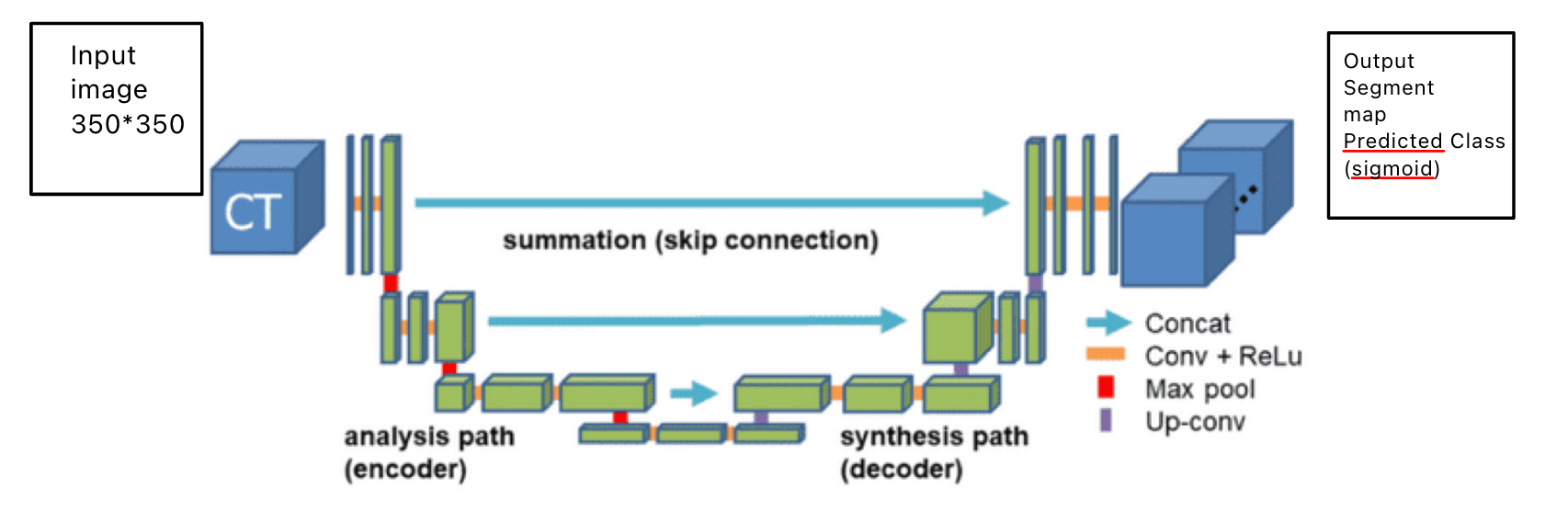
A UNET is generally composed of three distinctive blocks: a convolution operation, an encoder structure, and a decoder structure. The convolution operation is used as a building block and consists of two convolution layers, batch normalization and ReLu activation function. The encoder part takes an input tensor and applies the convolution operation followed by max pooling to return the output of the convolution block and the max-pooled output. The max pooling helps capture large receptive fields and reduces spatial dimensions. The decoder part is responsible for taking the input tensor and a skip connection tensor from the corresponding encoder block. The purpose of the skip connection is to allow the network to combine low-level features from the encoder with high-level features from the decoder enabling better localization and segmentation accuracy. Finally, the model then performs a couple of transformation operations before applying the convolution operation which is responsible for outputting a decoded feature map. To avoid a bias towards the majority class leading to poor performance, we used a dice loss function to maximize the dice coefficient by measuring the overlap between the predicted(p) and ground truth image mask(y). The dice loss is defined by:
Contribution:
The main purpose of our project was to tackle current issues specified by previous Kelp detection algorithms such as
the potential interference of occasional clouds in the detection of kelp forests due to changes in reflectance and the
high variability in the spatial patterns of kelp forests. We expect a UNet architecture to perform better because of its
data efficiency requiring fewer training samples compared to other image segmentation algorithms. Also, the skip connection
functionality of UNET enables the model to capture fine details and contextual information for precisely detecting kelp.
Furthermore, UNET has been specifically designed for image segmentation purposes and thus allows accurate representation of kelp patches within the image.
We expected our approach to solve the limitations of the literature by using data augmentation during the training to enhance the model’s robustness to cloud interference and spatial variability in kelp patterns. Our model would also be robust to variability due to the skip connections and multi-level mature extraction provided by the UNET. By learning from diverse examples, the model can accurately differentiate kelp and other elements, even in images with varying spatial patterns (including clouds).
Visuals: Approach pipeline
Experimental setup
We arrived at the approach discussed in the Methods section through the following experiments:
- Model Architecture: We experimented with different neural networks for semantic segmentation.
- Model Parameters: We experimented with different loss functions e.g. binary cross-entropy and our custom dice_loss function to train our neural network. We also tried out different values for the learning rate, optimizer, model depth, etc.
- Data Preprocessing: We experimented with different data pre-processing methods such as the use of the Normalized Difference Water Index (NDWI)[10] or the Normalized Difference Vegetation Index (NDVI)[11] parameters which are both used for determining the presence/absence of vegetation. The most appropriate data pre-processing techniques will be chosen based on the accuracy values recorded when the processed data is used to train our model.
By optimizing the model architecture and parameters, as well as the data preprocessing methods, we should arrive at a model that accurately maps kelp in satellite images.
To implement our method for kelp segmentation of satellite images, we made use of the dataset from the ‘Kelp Wanted: Segmenting Kelp Forests’ competition on the driven data website [12]. The training set includes 5,635 TIFF images/label pairs, and the test set includes 1,426 TIFF images. Each image/label has a size of 350x350 pixels, with the input image having 7 channels and the label having 1 channel (binary mask of kelp or no kelp). The 7 channels of the input image are described below.
- Short-Wave Infrared (SWIR): The SWIR band is highly useful for differentiating between water and land. Water bodies absorb more SWIR light, appearing darker, which can help distinguish kelp, which might reflect slightly more SWIR than plain open water. Near-Infrared (NIR): NIR is generally absorbed by water but reflected by vegetation. Kelp forests will likely show higher reflectance in this band compared to the surrounding water, making NIR a critical channel for identifying aquatic vegetation.
- Red (R): The red band is absorbed by chlorophyll in healthy vegetation, making it less reflective in vegetation-rich areas but more reflective in areas without vegetation. However, underwater, the red light is absorbed quickly, which might reduce its utility unless the water is very shallow.
- Green (G): This band might be helpful in mapping shallow underwater habitats since it can penetrate deeper than the red channel. The green color also gets absorbed by the natural green color of the kelp.
- Blue (B): Blue light penetrates deeper into the water than other visible wavelengths, which can help in identifying deeper kelp forests.
- Cloud Mask: The cloud mask is useful for preprocessing to eliminate areas obscured by clouds from your analysis, ensuring that only clear observations of the water and kelp are considered.
- Elevation: An elevation map (ground mask) serves as a ground mask by identifying land areas. We can utilize this map to exclude these land areas from the regions considered for kelp presence, ensuring more accurate prediction results.
- NDVI (Normalized Difference Vegetation Index): NDVI is calculated using the formula: NDVI = (NIR−Red)/(NIR+Red) where NIR is the near-infrared light reflected by vegetation, and Red is the visible red light reflected by the vegetation. NDVI values range from -1 to +1, where higher values indicate greater levels of live green vegetation, making it essential for assessing plant health and biomass.
- NDWI (Normalized Difference Water Index): NDWI is often calculated using one of two formulas depending on the specific application. NDWI = (Green−NIR)/(Green+NIR) where Green represents green light reflectance. This index helps differentiate water from terrestrial vegetation and is crucial for studies related to surface water mapping.
Due to the unavailability of the ground truth labels for the test set, we split the training set by a ratio of 70-15-15 for training, validating, and testing our model. Sample images of the RGB channels, NIR, SWIR, Cloud Mask, Elevation map, and label are shown below:
The desired output of our model is a binary mask/image with 0 representing the absence of kelp and 1 representing the presence of kelp. A sample output can be seen in the picture titled ‘Kelp Label’.
For evaluating our approach, we made use of the dice coefficient and mean Intersection over Union metrics as these work well with highly class imbalanced datasets as is common in semantic segmentation tasks.
Results
The example of visual output (qualitative) results are shown in the images below:
|:–:|
| Image Showing the example image – ground truth - predicted |
For the baseline results comparison, we will compare our results to the baseline established by the study “[5] Automated Satellite Remote Sensing of Giant Kelp at the Falkland Islands (Islas Malvinas).” This baseline indicates that the automated DTM algorithm performed nicely, producing labels closely aligned with the ground truth (expert-labeled). However, the automated KD algorithm did not perform as well, with its results significantly deviating from the expert labels.
Upon quantitative evaluation, the DTM algorithm demonstrated performance that matched or surpassed our model. Both the DTM and our U-Net model exhibited minor variations in size and slight deviations from the ground truth, with occasional over-labeling or under-labeling. In contrast, the KD algorithm underperformed relative to the DTM and exhibited performance that was either comparable to or worse than our model, often failing to accurately identify kelp on the satellite images.
|:–:|
| Image Showing the results from the paper: Automated satellite remote sensing of giant kelp at the Falkland Islands (Islas Malvinas) [5] |
Additionally, the table containing the input channel combination and quantitative results (mIOU + Dice) are shown in the table below:
Here are some thought processes, insights, and conclusions from the experiment:
- Initial Approach: We began by feeding the model basic visual RGB inputs, akin to what the human eye perceives. However, the results were suboptimal, indicating the need for more sophisticated satellite image data.
- Importance of NIR: Through research and practical observation, we identified the Near-Infrared (NIR) channel as crucial due to its high sensitivity to vegetation. NIR images provided clear and useful visual data, underscoring its significance.
- Inclusion of NDVI and NDWI: Implementing the Normalized Difference Vegetation Index (NDVI) and the Normalized Difference Water Index (NDWI) significantly enhanced prediction accuracy. Their effectiveness is well-documented in remote sensing, agriculture, and forestry, which we confirmed through our tests.
- Optimal Channel Configuration: The most effective input configuration at the time involved three channels: NDVI, NDWI, and NIR. The addition of a fourth channel, either Green or Blue, further improved the Dice coefficient, with Blue outperforming Green. This suggests that the Blue channel may better capture deeper, less visible kelp, possibly due to its penetration capabilities beyond what the Green channel can achieve.
- Channel Optimization: We found that incorporating both Green and Blue as fourth and fifth channels actually reduced model accuracy. Consequently, a four-channel input comprising NDVI, NDWI, NIR, and Blue yielded the best results, achieving a Dice coefficient of 0.536 and an mIOU of 0.993.
- Project Milestones and Future Directions: Achieving a Dice coefficient above 0.5 marks a project’s success within our current scope and timeline. However, while promising, the accuracy level is not yet sufficient for real-world application. Further refinement and development are required to enhance the model’s reliability and applicability.
Key Result Performance for Model:
Since this project is concerned with semantic segmentation, we determined that a UNet architecture would be appropriate because it can be adapted to multi-channel images of different shapes and it has a contractive and expansive network that helps us classify and locate kelp in the images. Multiple variations of the UNet architecture were tried, one of which is UNet with a ResNet50 encoder. Ideally, the use of the ResNet50 encoder should improve the feature extraction capabilities of the model. We also experimented with an ensemble of detectors (UNet model and ResNet50 model modified for semantic segmentation). The dice coefficient values of each of these architectures when trained/tested on input data with NDVI+NDWI+NIR channels can be seen below:
- UNet with a ResNet34encoder - 0.432
- Ensemble of UNet and ResNet50 - 0.48
- UNet - 0.52
Of these three models, the UNet model described in our Methods section performed best based on our evaluation metrics. The under-performance of the ensemble and ResNet50+UNet models may be attributed to inadequately tuned parameters.
Key Result Performance for Model Parameters:
The dice coefficient values of the different learning rates and loss functions tried when trained/tested on input data with NDVI+NDWI+NIR channels can be seen below: Loss function: The dice loss was chosen over the binary cross entropy loss due to its performance.
- Dice Loss - 0.52
- Binary Cross Entropy - 0.45
- Learning rate: A learning rate of 5e-3 was chosen over 1e-3 due to its performance.
- 1e-3 - 0.485
- 5e-3 - 0.52
Discussion
In summary, our project focused on the development of an approach for segmenting kelp in satellite images. We made use of UNet as our model architecture and the Normalized Difference Vegetation Index (NDVI), Normalized Difference Water Index (NDWI), Near Infrared channel (NIR), and Blue channel as our model input. With this approach, we attained a dice coefficient accuracy of 0.536. While this value indicates that the model can classify kelp a majority of the time, it is not satisfactory for real-world applications and does not outperform the approaches discussed in our related works section.
Through this project, we have learned the following:
- The default accuracy metric in Scikit- learn may not be appropriate for semantic segmentation tasks and will likely give an inflated accuracy value as it does not penalize false positives.
- Properly tuned parameters can significantly improve the performance of your neural network.
- Data preprocessing such as utilizing the cloud and ground channels, along with combining different hyperspectral data can also significantly improve the performance of the neural network as can be seen from the results of our experiment.
- Scientific knowledge in remote sensing. We learned the benefits of each satellite image channel and how to utilize them for the analysis of the hyperspectral image for environmental monitoring.
Additionally, we have also learnt how to build and combine layers of networks to perform semantic segmentation. If we were to start over today, we would increase the complexity of our model so that it learns more from the input data. We would also consider starting the training step earlier so that we could explore more computationally demanding models and have enough time to run them. We would also invest more time in the initial phases of the project to manually detect and correct/remove data corruption in satellite images or develop algorithms to detect them automatically.
For future work, we can explore these options:
- Implement manual or automated techniques to identify and remove corrupted satellite images, which are detrimental to model performance.
- Experiment with more complex versions of the U-Net architecture to enhance the model’s capability to segment kelp accurately.
- Employ a broader range of data augmentation techniques, such as flipping, random scaling, elastic deformations, and random rotations. These methods can help generalize the model better and reduce overfitting by simulating a variety of imaging conditions.
- Explore options for automating hyperparameter tuning to systematically improve model performance.
- Deploy the model in real-world settings to evaluate its practical effectiveness and reliability. Recording and analyzing the results from actual field tests will provide valuable insights that can be used to further refine the model.
Challenges Encountered
- Computational power: Due to the complexity of the model and the extensive size of the dataset, training requires substantial RAM and considerable computational resources. This intensive demand can significantly impact the runtime, necessitating the use of better computers and GPUs. We tried using the PACE cluster but ran into multiple issues. We decided to pursue Google Colab which was enough since we were running out of credits.
- Exceeding 0.55 dice coefficient: Despite experimenting with various model architectures and combinations, we struggled to achieve a Dice coefficient exceeding 55%. This threshold highlights potential limitations in our model’s architecture or the need for further optimization of our training processes.
- Error in the dataset: During a detailed manual inspection and survey of the dataset, we discovered that numerous satellite images were corrupted. These corruptions manifest as unexpected artifacts, such as white tabs, grids, or blackout areas, obscuring critical details of the land and water features represented in the images. These might be one of the culprit in reducing the model’s performance.
Team member contributions:
Nadira Amadou:
- Tuneed hyperparameters for UNET
- Implemented a UNET architecture with a Resnet 34 backbone
- Looked into Mask RCNN implementation
Contributed in reportOluwatofunmi Sodimu:
- Tuned hyperparameters for UNET
- Implemented UNET architecture with Resnet
- Looked into Mask RCNN implementation
- Contributed in report
Thanapol Tantagunninat:
- Tested different Data augmentation Techniques on the model
- Tuned and Tested different hyperparameters
- Contributed in report
References
[1] Kelp Forest. Kelp Forest | NOAA Office of National Marine Sanctuaries. (n.d.). https://sanctuaries.noaa.gov/visit/ecosystems/kelpdesc.html
[2] Browning, J., & Lyons, G. (2020, May 27). 5 reasons to protect kelp, the West Coast’s powerhouse Marine Algae. The Pew Charitable Trusts. https://www.pewtrusts.org/en/research-and-analysis/articles/2020/05/27/5-reasons-to-protect-kelp-the-west-coasts-powerhouse-marine-algae#:~:text=3.-,Protect%20the%20shoreline,filter%20pollutants%20from%20the%20water.
[3] NASA Earth Observatory. Monitoring the Collapse of Kelp Forests. https://earthobservatory.nasa.gov/images/148391/monitoring-the-collapse-of-kelp-forests
[4] Marquez, L., Fragkopoulou, E., Cavanaugh, K.C. et al. Artificial intelligence convolutional neural networks map giant kelp forests from satellite imagery. Sci Rep 12, 22196 (2022). https://doi.org/10.1038/s41598-022-26439-w
[5] Automated satellite remote sensing of giant kelp at the Falkland Islands (Islas Malvinas) Houskeeper HF, Rosenthal IS, Cavanaugh KC, Pawlak C, Trouille L, et al. (2022) Automated satellite remote sensing of giant kelp at the Falkland Islands (Islas Malvinas). PLOS ONE 17(1): e0257933. https://doi.org/10.1371/journal.pone.0257933
[6] Finger, D. J. I., McPherson, M. L., Houskeeper, H. F., & Kudela, R. M. (2020, December 17). Mapping Bull kelp canopy in northern California using landsat to enable long-term monitoring. Remote Sensing of Environment. https://www.sciencedirect.com/science/article/pii/S0034425720306167#:~:text=Past%20efforts%20to%20estimate%20kelp,et%20al.%2C%202006
[7] Mahmood A, Ospina AG, Bennamoun M, An S, Sohel F, Boussaid F, Hovey R, Fisher RB, Kendrick GA. Automatic Hierarchical Classification of Kelps Using Deep Residual Features. Sensors. 2020; 20(2):447. https://doi.org/10.3390/s20020447
[8] Uhl, F., Bartsch, I., & Oppelt, N. (2016, June 8). Submerged kelp detection with hyperspectral data. MDPI. https://www.mdpi.com/2072-4292/8/6/487
[9] Unet diagram
[10] Gao, B.-C., Hunt, E. R., Jackson, R. D., Lillesaeter, O., Tucker, C. J., Vane, G., Bowker, D. E., Bowman, W. D., Cibula, W. G., Deering, D., & Elvidge, C. D. (1999, February 22). Ndwi-a normalized difference water index for remote sensing of vegetation liquid water from space. Remote Sensing of Environment. https://www.sciencedirect.com/science/article/abs/pii/S0034425796000673
[11] GISGeography. (2024, March 10). What is NDVI (normalized difference vegetation index)?. GIS Geography. https://gisgeography.com/ndvi-normalized-difference-vegetation-index/
[12] DrivenData. (n.d.). Kelp wanted: Segmenting kelp forests. https://www.drivendata.org/competitions/255/kelp-forest-segmentation/page/792/